SQL Server 2012 Analysis Services Tabular Models

The recent SQL Server 2012 release (formerly codenamed Denali) is accompanied, as usual in any new version, for several interesting improvements. In this article we’ll focus on development of analytical tabular models, an integral part of Business Intelligence Semantic Model (BISM), the new paradigm for developing Business Intelligence (BI) solutions based on SQL Server 2012 Analysis Services.

As was already mentioned in the introductory article about PowerPivot, the incorporation of BISM into Analysis Services makes SQL Server one of the most powerful solutions within the current BI arena. However, since the first public announcements about BISM so far, new details have been revealed about the architecture of this technology, allowing us to be more precise in the descriptions of it.

 

BISM. A single model for all analytical needs

BISM becomes the new model for the development of BI solutions that fulfills the analysis requirements of all kind users.

BISM represents an evolution from Unified Dimensional Model (UDM) towards a combined model that offers all UDM multidimensional development features plus new features based on a relational analysis engine, what enrich the current SQL Server offer in the analytical services area. Therefore, from now on, the term UDM is replaced for BISM, when we mention the development model used by Analysis Services. Similarly, when we update an UDM project to SQL Server 2012, it will be deemed as a BISM project for all purposes.

This integration between work philosophies, and hence on the underlying technologies (multidimensional and relational), results in an architecture distributed in three layers, as we see in the following image, with response capacity to users with very different needs in all concerning tasks related to data analysis.

 

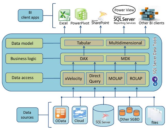
Watching the workflow of this architecture in a bottom-top direction, in first place, we find the data access layer, which is responsible for performing the information extraction resident in the data sources we connect, existing two modes for this extraction: cache and passthrough.

The caching mechanism gets the data from the original source and stored it in a data structure based on a compression algorithm optimized for high-speed access. In turn, using this cache mode we must choose two different storage engines: MOLAP or xVelocity.

MOLAP is the intermediate storage system traditionally used in Analysis Services, and as the name suggests, is optimized for use in multidimensional models development (OLAP cubes).

xVelocity is a brand new system introduced with BISM for use in tabular models, consisting of a column based data storage engine, which combines sophisticated compression and search algorithms, to offer, without using indexes or aggregations, excellent performance in speed response to our queries.

Regarding to passthrough mode, as its name implies, sends the query directly to data source engine, so both operations: data processing and business logic are performed there. In this case there are two modes of execution too: ROLAP and DirectQuery.

ROLAP mode is usually used by Analysis Services, which uses the data source itself to process queries against cubes belonging to multidimensional models.

DirectQuery is used in tabular models to also process queries in the data source.

Business logic layer includes queries in MDX ​​or DAX languages with which we’ll implement our solution’s logic, depending whether we work respectively against a multidimensional or tabular model.

Finally, in the data model layer we find the conceptual part of this architecture, where using SQL Server Data Tools (formerly Business Intelligence Development Studio and current development environment based on Visual Studio 2010) will build our model using one of the available project templates: Analysis Services Multidimensional and Data Mining Project or Analysis Services Tabular Project.

It’s worth mentioning that it is also possible to use PowerPivot as development tool for a tabular model, but to deploy it in the server it’s mandatory to use SQL Server Data Tools.

 

Installing Analysis Services. A semantic model, two modes of execution

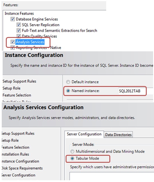
Due to the particular features of each BISM data model, in SQL Server 2012 setup, at Analysis Services step, we must choose which analysis server execution mode we want to install: Multidimensional or Tabular, because it is not possible to install both simultaneously in the same instance. For this reason the recommended procedure is to install separate instances. However, in our case it is sufficient to install only the tabular mode for the development of this example.

 

Let’s get started. Creating a tabular model

Exposed all necessary aspects to conceptually locate the reader within the new semantic model, let’s get into the practical part of the article, in which we will develop a tabular analysis project.

We will use the sample database AdventureWorksDWDenali being the model’s goal to analyze the shipping orders expenses placed by customers through the Internet and the number of orders issued, all according customer’s residence location and promotion details about items purchased.

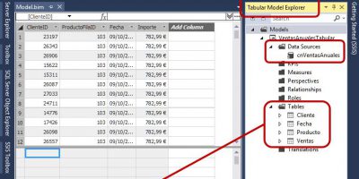
In first place we will start SQL Server Data Tools, creating a new project based on Analysis Services Tabular Project template, giving it the name PruebaModeloTabular. As we shall see in Solution Explorer, this project will consist of a file named Model.bim, which represents the tabular model designer.

 

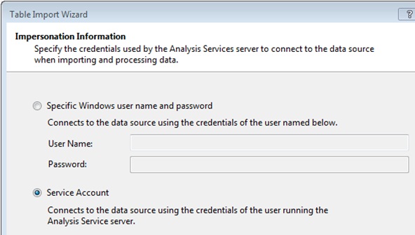
The next step will be to add tables to the model, so we’ll select the menu option «Model | Import From Data Source», which will start the data import wizard. After choosing the type of data source, SQL Server instance and database, we reach the step where we must enter credentials to connect to the data source and proceed with data extraction.

At this point we’ll use our Windows account (in case we have adequate access permissions) or choose the Service Account option, which will use the NT SERVICEMSOLAP$SQL2012TAB account (SQL2012TAB is the SQL Server instance name of my machine) associated with the Analysis Services service. If we use the latter possibility, we need to grant access and read permissions to this account on the AdventureWorksDWDenali database.

 

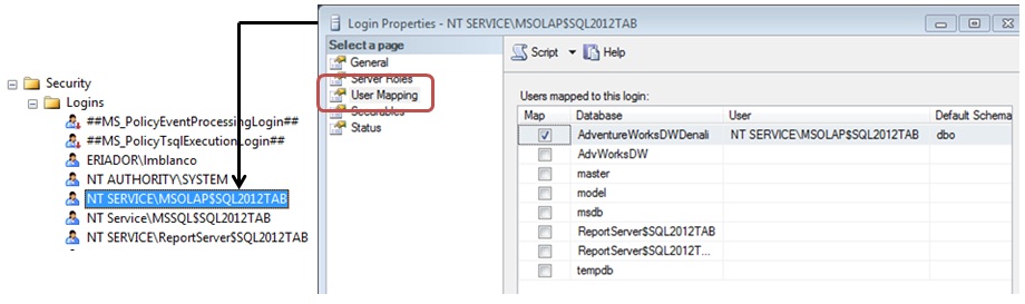
To assign that permission, in SQL Server Management Studio we right-click the Logins node, belonging in turn to Security node, choosing New Login option, which will open the dialog box to add a new login to the server, where we’ll type the Analysis Services account name. In User Mapping section we’ll check the database to grant access.

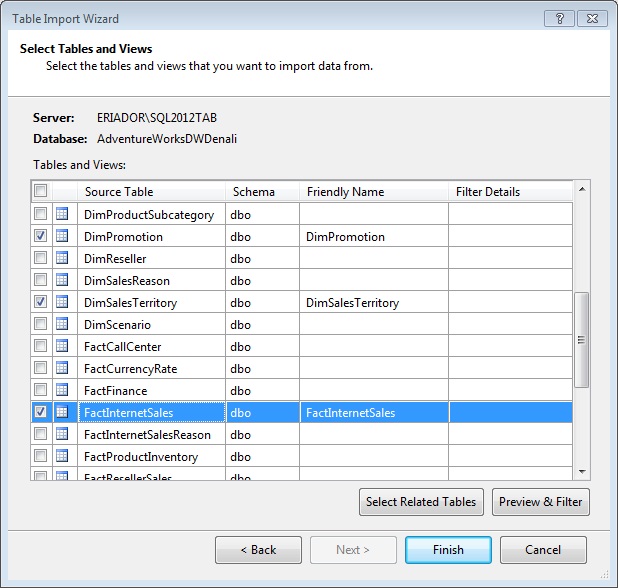
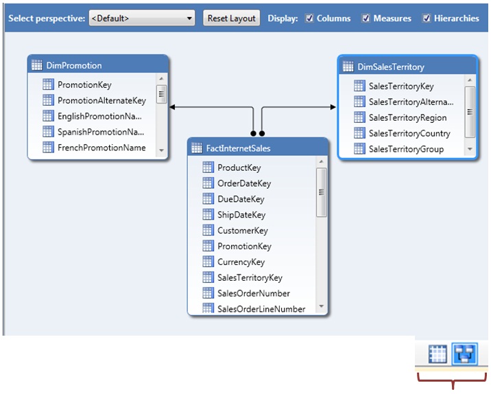
Continuing the import wizard we’ll reach the selection table step, where we’ll check DimSalesTerritory, DimPromotion and FactInternetSales tables, and proceeded to start the import process.

 

When the data import process finishes, the designer will show the tables in a grid, arranging them into tabs.

 

This display mode can be switched to a diagram mode, more suitable if we want to focus on concrete elements such as relationships between tables. To change the view mode use the buttons for that purpose in the bottom right of the designer window.

 

Creating measures

Despite having imported tables to the model, we still can’t conduct a proper analysis on it, because we lack the calculations (measures in BI context) responsible for providing numerical results, essential in any system of this type, as we saw in the article about OLAP Cubes.

To create a measure for the model, we must firstly set the designer’s display to grid (default mode). Once this adjustment is made, we see that each table shows two sections: top, which contains the rows of the table itself, and bottom, reserved for calculated measures created by the model developer.

Next we’ll select the FactInternetSales table (also known as fact table in multidimensional context) that contains those columns that can be used in obtaining numerical results.

We will use the Freight column to create the first of our measures: sum of the values ​​in that column for table’s rows. In grid’s bottom area we’ll select an empty cell for the column above mention, then we’ll click the toolbar’s Sum button, which apply the DAX language formula «SUM([Freight])» to the column.

As a result of this operation we’ll obtain the Sum of Freight measure, but we’ll change this name, assigned automatically by the development environment, to GastosTransporte, using the properties window.

 

Watching the resulting figure we will realize that there’s a formatting problem with the obtained value (7,339,696,091.00 €), as the correct result is 733969.6091. We can verify this running the following query in SQL Server Management Studio.

SELECT SUM(Freight) FROM FactInternetSales
 

 

However, we’ll find this difficulty only in model designer scope, since as we shall see in the next section, when analyze it from an external tool, the values ​​are displayed correctly.

Next we will create the measure to calculate the orders quantity issued by the company, so we’ll apply to SalesOrderNumber column a distinct count operation, because the FactInternetSales table can have more than one row for the same order.

We can drop-down the Sum button in Visual Studio’s toolbar, so we can choose some of the most common calculations, Distinct Count among them, but this time we’ll manually create the measure FacturasEmitidas, writing the DAX following expression in the formula bar.

 

FacturasEmitidas:=DistinctCount([SalesOrderNumber])

 

Analyzing the model from Excel

If we have Excel 2010 installed we can use it as analysis tool for the model we are developing. All we have to do is select the menu option «Model | Analyze in Excel» and Visual Studio will open Excel, loading the model in a PivotTable.

On the pivot table panel PivotTable Field List we will check the GastosTransporte measure, which will be located in the block Values. Similarly we’ll proceed with SpanishPromotionCategory field from DimPromotion table, but this time we’ll place it on Column Labels block. Finally, fields SalesTerritoryGroup and SalesTerritoryCountry from DimSalesTerritory table will be placed in Row Labels block, so that we can watch this information into a hierarchical fashion.

 

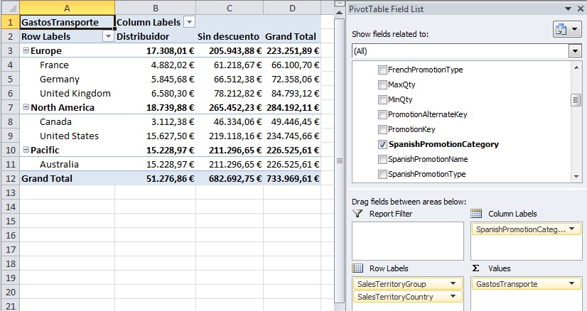
At the same time we can analyze the amount of bills issued by the company for sold items, adding FacturasEmitidas measure to the PivotTable, so we also get this information by the fields currently located in rows and columns or by other fields belonging to the model.

Those readers who have had the opportunity to use PowerPivot will find interesting similarities with this way of work, since in both cases the underlying technology is the same.

 

Conclusions

Tabular analysis models belonging to BISM, the new paradigm in building BI solutions, shipped with SQL Server 2012, are a great tool to develop powerful information systems using SQL Server Analysis Services. In this article we have made ​​an introduction to this interesting technology, showing the reader how to take advantage from it.