
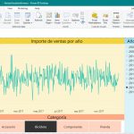
SSAS Tabular, SSIS y Power BI en acción. Elaboración de informes con Power BI Desktop
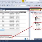
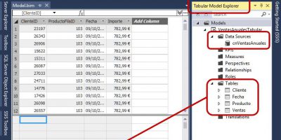
SSAS Tabular, SSIS y Power BI en acción. Modelo tabular. Diseño y carga de datos
SSAS Tabular, SSIS y Power BI en acción. Dimensiones. Fecha
SSAS Tabular, SSIS y Power BI en acción. Tabla de hechos. Unificación de operaciones de cálculo aleatorio
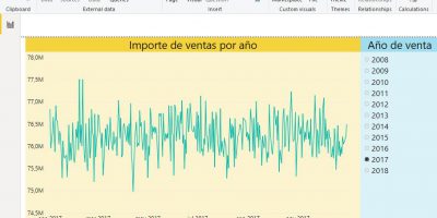
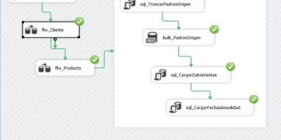
SSAS Tabular, SSIS y Power BI en acción. Tabla de hechos. Carga masiva de datos